Accelerating a Diffusion Simulation
Program performance has always been a topic of interest for me, but not something I've been able to explore very much outside of a class or two. I finally got around to it! Kind of. I decided to write a 2D heat diffusion simulation in a bunch of different ways, and compared their performance. All code is available on Github. First, a quick visualization:
The Math
Since wssg doesn't support LaTeX yet, the discretization of the diffusion equation is on Github.
Implementations
I've loosely described all the implementations below, along with code snippets and the occasional foreword on their performance.
aux is all the constant terms bundled together into one.
Python Naive
The naive Python implementation is the most straightforward one to implement I could think of; it iterates over each element of the 2D array, and updates the value of that element based on the central finite difference scheme described above.
# c, the 2d array
for _ in range(num_steps):
    for i in range(1, len(c) - 1):
        for j in range(1, len(c[0]) - 1):
            c_tmp[i][j] = (c[i][j] + aux *
                            (c[i - 1][j] + c[i + 1][j] +
                            c[i][j - 1] + c[i][j + 1] -
                            4 * c[i][j]))
    c, c_tmp = c_tmp, c
Python NumPy
Exactly the same as the naive python implementation above, but using NumPy arrays instead of Python lists. As the results section will show, this is actually slower than the basic Python, which makes sense: we're not doing what NumPy is good at, which is making a single call to a NumPy function, then letting its highly-optimized C backend perform the longer running operation. Instead, we're indexing an array and performing some basic arithmetic, which involves lots of calls through NumPy to the underlying C structures and functions, and that's about it; it's all overhead.
# c, the 2d array
for _ in range(num_steps):
    for i in range(1, len(c) - 1):
        for j in range(1, len(c[0]) - 1):
            c_tmp[i][j] = (c[i][j] + aux *
                            (c[i - 1][j] + c[i + 1][j] +
                            c[i][j - 1] + c[i][j + 1] -
                            4 * c[i][j]))
    c, c_tmp = c_tmp, c
Python SciPy
One of my roommates pointed out that the forward scheme we're using is essentially just convolving by a 3x3 kernel, which opens up a whole world of options in Python that make more sense, namely the "call a single function that's running optimized C underneath" described above.
The first of these implementations is using SciPy's signal.convolve2d method.
Since the backend isn't in Python, we should get a hefty speedup relative to our naive Python implementation; I'm curious if it'll beat my naive C++ implementation (described below).
kernel = aux * np.array([[0, 1, 0], [1, -4, 1], [0, 1, 0]])
for _ in range(num_steps):
    c_tmp = c + np.pad(
        scipy.signal.convolve2d(c, kernel, mode='valid'),
        1, 'constant')
    c, c_tmp = c_tmp, c
Python CuPy
CuPy is a library which provides functions found in NumPy and SciPy, but designed to run on the GPU instead of CPU, so instead of calling scipy.sigsnal.convolve2d, we call cupyx.scipy.signal.convolve2d.
This makes it a great candidate for comparing against the CUDA implementation provided below.
Again, I'm curious to see how my fairly straightforward/unoptimized CUDA approach compares to this.
kernel = aux * cp.array([[0, 1, 0],[1, -4, 1],[0, 1, 0]])
for _ in range(num_steps):
    c_tmp = c + cp.pad(
        sgx.convolve2d(c, kernel, mode='valid'),
        1, 'constant')
    c, c_tmp = c_tmp, c
Python Torch
PyTorch also provides functions for convolving tensors (generic N-dimensional arrays) on a GPU, so we can compare how well CuPy and Torch perform with respect to each-other, but also with respect to my CUDA implementation.
# skipped some unsqueezing to make them 4D as required
kernel = aux * torch.tensor([[0, 1, 0],[1, -4, 1],[0, 1, 0]],
                            dtype=torch.float64,
                            device=gpu)
for _ in range(num_steps):
    c_tmp = c + torch.nn.functional.pad(
        torch.nn.functional.conv2d(c, kernel, padding='valid'),
        (1,1,1,1), 'constant', 0)
    c, c_tmp = c_tmp, c
C++ Naive
Essentially the naive Python implementation, but ported over to C++. As we'll see, trying to perform lots of arithmetic in pure Python without dropping down to C in the backend has pretty abysmal performance, and I don't think it's too much of a stretch to say that no reasonable high-performance program would use pure Python. This implementation is therefore what I will call our 'baseline', a reasonable approach to solving our problem, if not unoptimized.
Something that didn't make it into the final benchmark was the use of optimization flags.
With D = 0.1, L = 2.0, N = 200, and T = 0.5, I got a runtime of 1.1 seconds without the use of -O3, and 0.048 seconds with it, an over 20x speedup.
Short moral of the story: let the compiler do its magic.
// M is the array width with the padding/border of zeros
// (boundary condition)
for (size_t step = 0; step < num_steps; ++step) {
    for (size_t i = 1; i < M - 1; ++i) {
        for (size_t j = 1; j < M - 1; ++j) {
            c_tmp[i * M + j] = c[i * M + j] + aux * (
                c[i * M + (j + 1)] + c[i * M + (j - 1)] +
                c[(i + 1) * M + j] + c[(i - 1) * M + j] -
                4 * c[i * M + j]);
        }
    }
    std::swap(c, c_tmp);
}
OpenMP
OpenMP is an API that allows for incredibly simple multithreading; instead of having to spawn threads, divide the workload manually based on the thread-id, then joint them at the end, we can #include , add a single #pragma parallel for collapse(2) statement which'll automatically spawn threads, distribute the work over the nested loops, then join them at the end for us.
For a perfectly parallelizable workload, doubling the number of cores should cut the execution time in half; as we'll see, central finite difference diffusion isn't even close to perfectly parallelizable, and so the actual speedup isn't as drastic.
I didn't mess with the number of threads, leaving it the default, which seems to be the number of cores.
#include
for (size_t step = 0; step < num_steps; ++step) {
    #pragma omp parallel for collapse(2)
    for (size_t i = 1; i < M - 1; ++i) {
        for (size_t j = 1; j < M - 1; ++j) {
            c_tmp[i * M + j] = c[i * M + j] + aux * (
                c[i * M + (j + 1)] + c[i * M + (j - 1)] +
                c[(i + 1) * M + j] + c[(i - 1) * M + j] -
                4 * c[i * M + j]);
        }
    }
    std::swap(c, c_tmp);
}
CUDA
A fairly naive port of my C++ and Python logic over to CUDA. Unlike OpenMP, we need to make a little bit more of an effort to distribute the work amongst all our streaming multiprocessors (SM). I went for the path of least resistance in my implementation: after a little experimenting, I settled on 32 threads per block and 32 times the number of SM of blocks to be distributed amongst the SMs. Each thread calculates the new value at its index, then jumps 32 32 SMs elements forward, and repeats until the end of the array is found.
__global__
void step_kernel(double *c,
                double *c_tmp,
                const double aux,
                const size_t M) {
    // skip first row (boundary condition)
    int index = threadIdx.x + blockIdx.x * blockDim.x + M + 1;
    int stride = blockDim.x * gridDim.x;
    // skip last row (boundary condition)
    for (size_t i = index; i < (M * M) - M; i += stride) {
        // skip first and last column (boundary condition)
        if (i % M != 0 && i % M != M - 1) {
            c_tmp[i] = c[i] + aux * (
                    c[i + 1] + c[i - 1] +
                    c[i + M] + c[i - M] -
                    4 * c[i]);
        }
    }
}
Test Setup
The benchmark was run on a laptop with an Intel Xeon W-10885M CPU and NVIDIA RTX 3000 GPU. The CPU was fairly top-of-the-line for laptops when it came out, while the GPU was more mid-range, performing a little worse than an RTX 2070 mobile. This model of laptop is known to struggle with thermal throttling, so while I haven't done anything to mitigate this, it's perhaps worth keeping in mind that tests which use more CPU cores or the GPU may perform better on a system with proper cooling. Finally, I'm running Ubuntu 22.04 and CUDA 12.0.
Each implementation was run with array widths varying from 16 to 1024 in powers of 2; very slow implementations were not run past array widths of 256. Each was only run once, which I'll have to go back and rectify at some point to.
Results
First, we can look at the overall execution time as a function of the array width for each implementation.
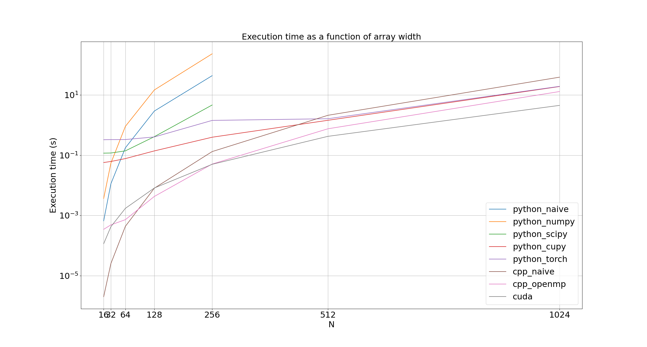
It's quite hard to grasp just how explosive the growth in execution time is due to the log scale on the y axis. Massaging the equations in the math section a little bit and assuming we're using the just-stable step size as described above, we find the number of steps as (see Github for LaTeX)
numsteps = (4DT ( N^2 - 2N + 1 right)) / (L^2) + 1
which means that if we fix the width of our problem L, the diffusion constant D, and the simulation time T, then the number of steps scales with the square of the array width N. Worse, each step requires iterating over an N times N array, so the total number of array elements to perform calculations on scales to the power of four of the array width N. Meaning every time we double the array size, our time to execute should be multiplied by 16. A slightly easier to interpret figure plots the speedup of each implementation compared to our naive, single-core C++ one.
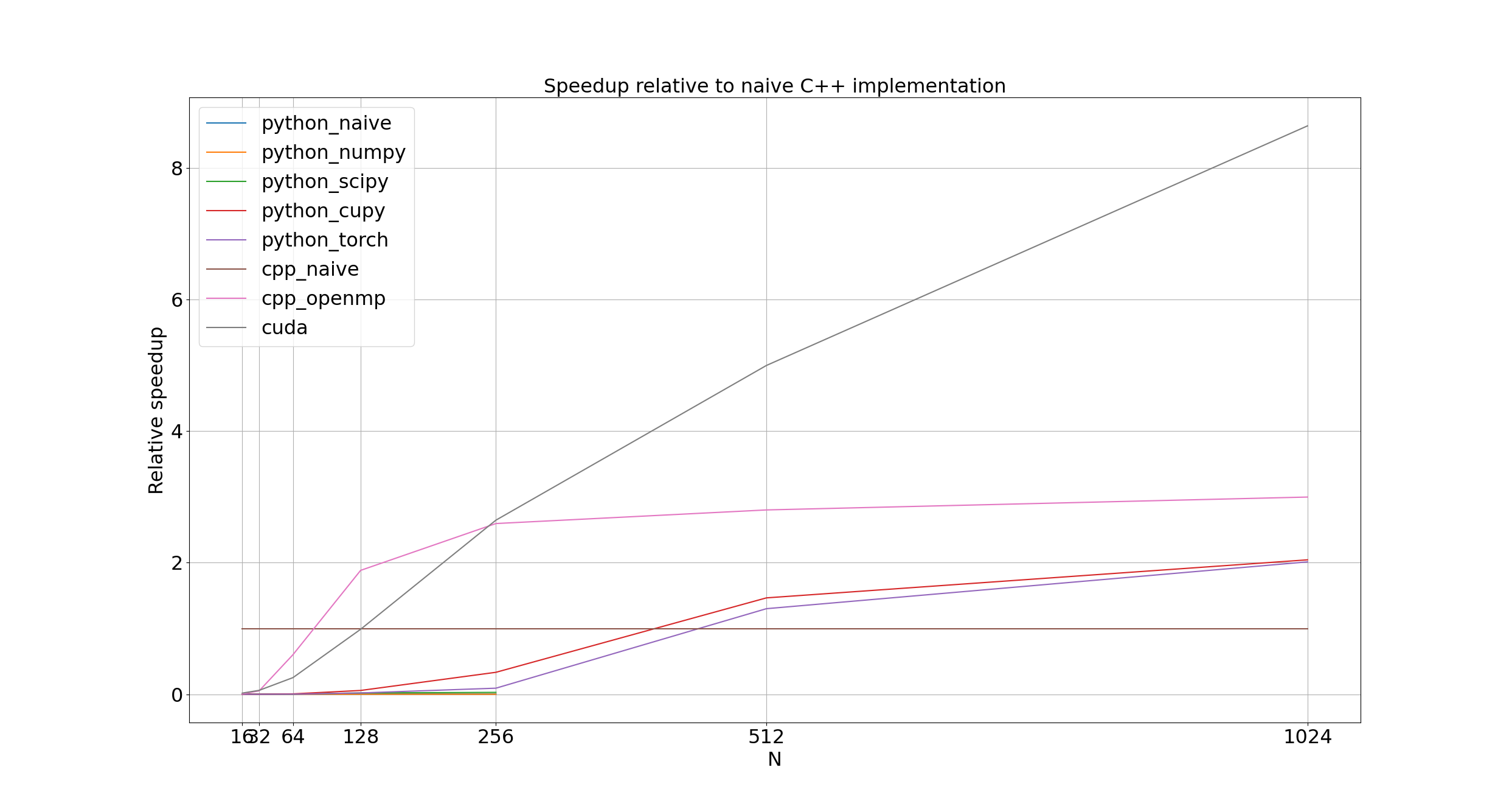
For arrays smaller than 128 by 128 elements, the naive C++ implementation (cpp_naive) dominates; beyond this, though, and all parallel implementations handily out-perform it.
OpenMP (cpp_openmp) only outperforms cpp_naive by about 50% at an array width of 128; once an array width of 256 is reached, it evens out to 3x cpp_naive's performance.
I suspect that the overhead of spawning and joining threads is still significant compared to the overall execution time for arrays less than 256 elements wide, but once we hit that size, the overhead becomes insignificant.
CUDA (cuda) is the real winner here, handily beating the cpp_naive for an array width of 128, crushing it and matching cpp_openmp for an array width of 256, then for any larger arrays, crossing the finish line, leaving the stadium, and hijacking a rocket to mars before the other approaches even leave the starting block.
Its lacklustre performance for smaller arrays is to be expected: with 32 threads per block and 960 blocks queued up across the streaming multiprocessors, that means 30 720 threads are being spawned for an array that has 16 384 (128 by 128) elements are less, meaning less time doing calculations, and more time checking to see if a given thread has an index within the bounds of the array.
A 256 by 256 array has 65 536 elements though, enough to give every thread a little bit of work and more.
The largest surprise for me were the CuPy (python_cupy) and Torch (python_torch) implementations; while I had the luxury of tuning the number of threads per block and blocks per grid of my CUDA code, I would have expected under-the-hood optimizations in both libraries to help them both outperform my pedestrian CUDA code.
Like cuda, perhaps their default thread and block numbers are suboptimal for small arrays, and only become -ish saturated later.
While both eventually found their footing at array widths 512 and outperformed cpp_naive, neither caught up to cpp_openmp, let alone cuda.
Am I holding it wrong, or is it the limit of what these generic implementations can do?
Notice the little lines in the bottom left? That's the corner of shame, for implementations that were too slow to bother running on arrays wider than 256.
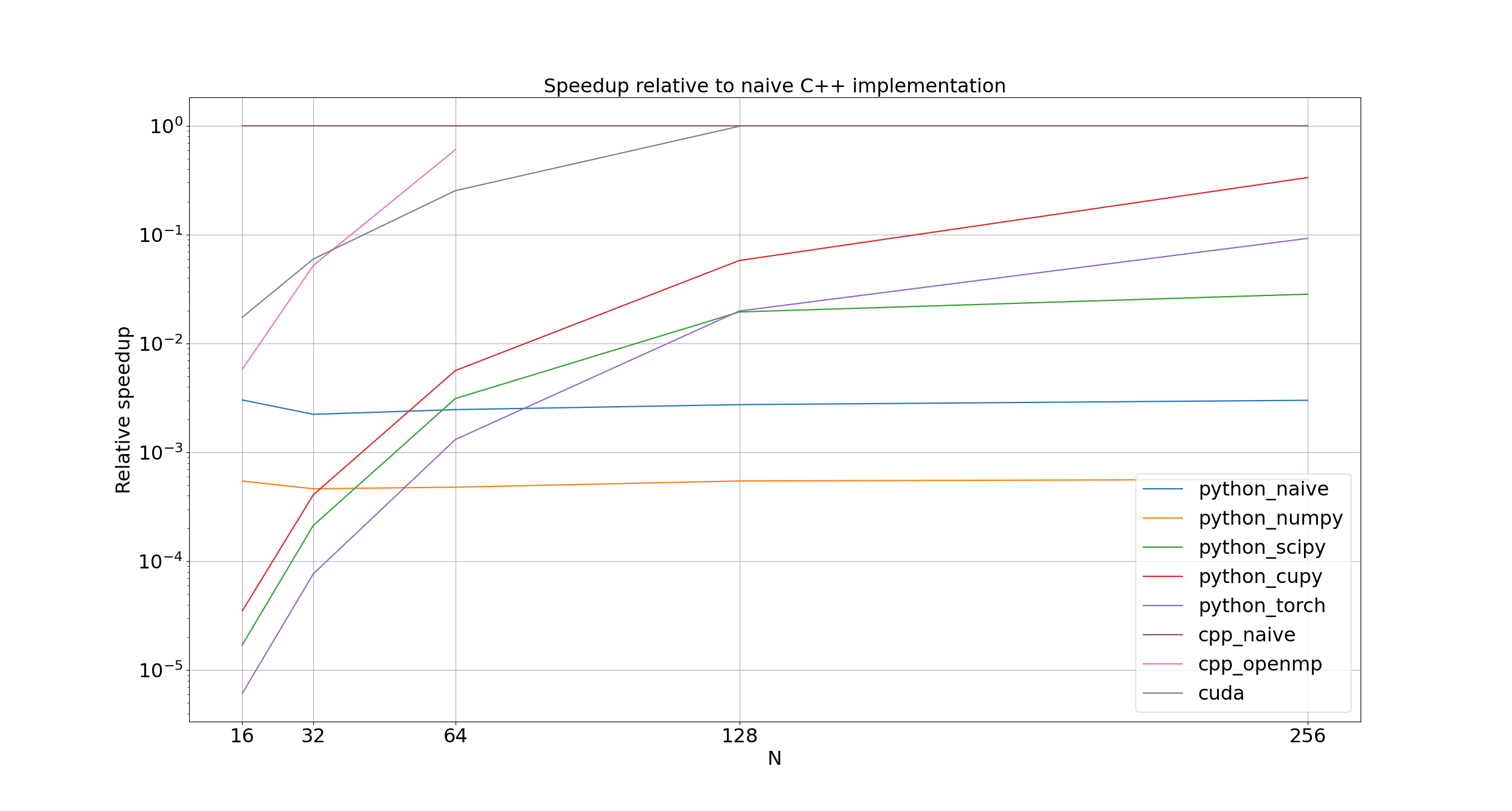
Unsurprisingly, the naive Python and NumPy implementations (python_naive and python_numpy) are between 100 and 1000 times slower than cpp_naive.
More surprisingly, SciPy (python_scipy) never comes within an order of magnitude of cpp_naive; I would have expected the C backend of scipy.signal.convolve2d to be at least competitive with my straight-forward C++ implementation.
Perhaps the number of extra features and function arguments slow it down significantly compared to my approach, where the padding handling is hard-coded and inflexible.
Perhaps this also explains why python_cupy and python_torch never reach the same performance as cuda.
Perhaps I just chose the wrong flags.
I didn't add the time to copy the arrays to and from the GPU for cuda, python_cupy, or python_torch.
I figured, if I were really trying to run this in more than a goofing-off setting, I would have initially allocated them on the GPU to start with.
For fun, here's the time required to move arrays to and from the GPU for cuda, compared to the execution time:
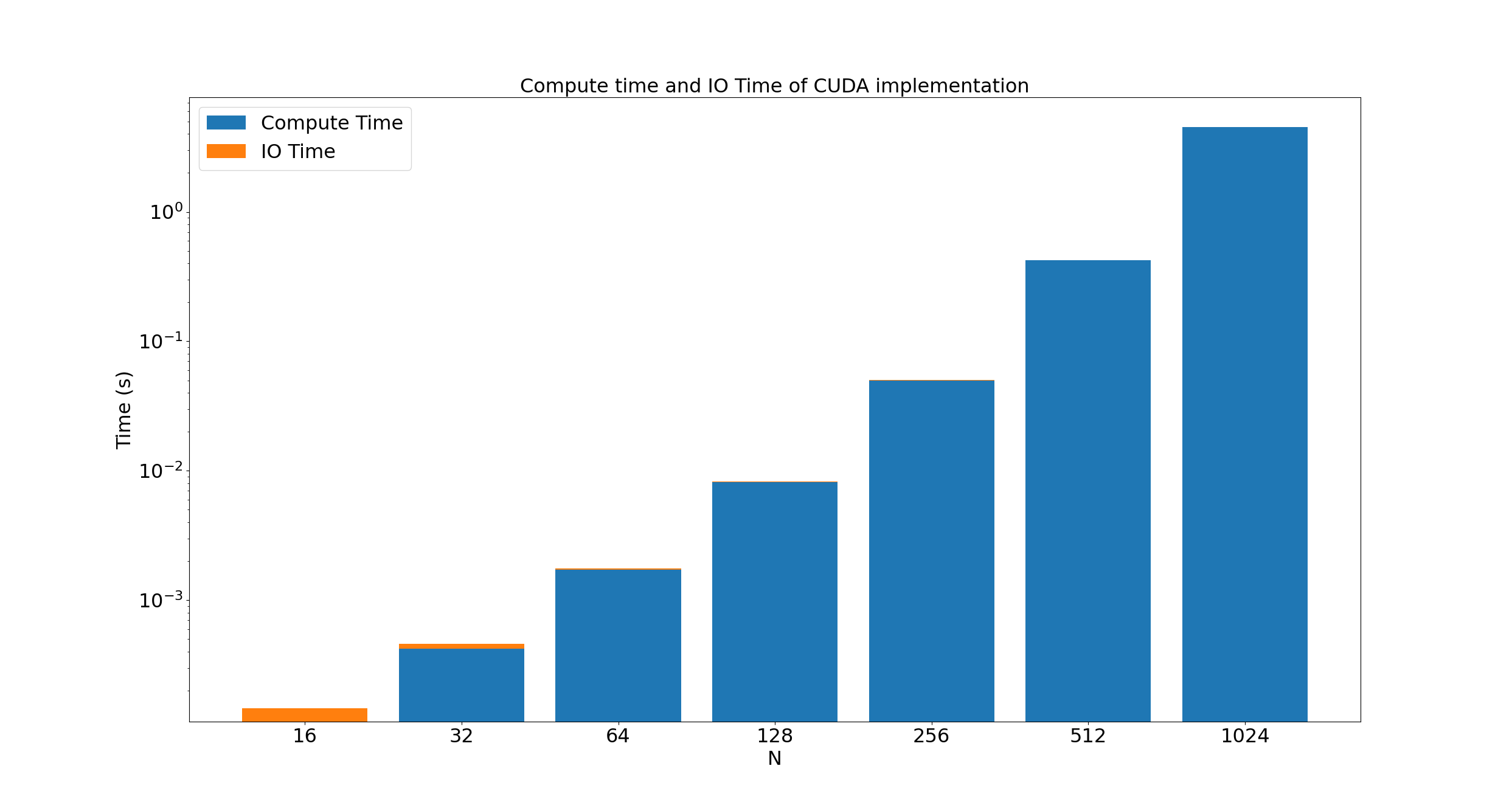
For very small arrays, the overhead of moving from the host to the device is significant, but as the array size doubles, the number of elements to move quadruples, and the number of calculations to make increases by 16; moving the arrays from the host to the device very quickly becomes insignificant.
Conclusions
As expected, writing any kind of high performance code in Python without calling C in the backend is going to be unbearably slow. I can imagine libraries like Torch, CuPy, and SciPy handily beating my C++ and CUDA code when the problem is right, but for this specific simulation, or at least for my programming lack-of-know-how, dropping down to C++ and CUDA gives the best results, at the cost of programming time, of course.
To Do
Oh gosh, there's a lot of things I'd love to try, and not enough time to do them all.
- Run each implementation multiple times and average the execution times
- Examine the effect of thread count on OpenMP performance
- Run using
floatinstead ofdouble, since this GPU has a 30:1 GFLOP ratio between the two (simply less 64-bit arithmetic units and registers) - Avoid padding operation for SciPy, CuPy, Torch, instead operating on array without padding then adding the paddindg back at the end
- CUDA version with dynamic shared memory and separate x and y derivates (maybe some fast transpose to improve memory coalescing for y derivatives?)
- C++ version with separate x and y derivates (maybe some fast transpose to improve spatial cache locality for y derivatives?)
- C++ version with omp simd or ivdep
- C++ version with manual vectorization (SIMD instructions, AVX)
- C++ version with manual vectorization and manual threading
- Parallelize Python code
- Look into isolating processes (some examples here)
- Give overview of OpenMP (incl. non-linear scaling), vectorization, CUDA (for example, physical architecture)
- Profile CUDA code
Lessons Learned
Some silly small things I wasted way too much time on while writing this.
- CUDA will throw
CUDA Runtime Error: an illegal memory access was encounteredif a reference is passed to a kernel - Declaring arguments as
constin a kernel is unecessary, as all values are passed as const